6 Renormalisation

So far, we have only considered the leading order (LO) in $\alpha$ or $\alpha_{s}$ . This can be sufficient for certain observables in QED but it rarely is good enough in QCD (since $\alpha_{s}\gg\alpha$ ) or if we are doing precision physics. This means we will need to go to higher orders in $\alpha$ . Luckily, we know how to do this! The Feynman rules are perfectly valid beyond LO and we have already mentioned that it is possible to construct diagrams with loops. The only problem is now that momentum-conservation at each interaction vertex is no longer sufficient to determine the momentum in each propagator. If you have a look at the diagram we had in (178), the photon momentum can take any value $k$ . This means that we need to integrate over all possible values of this unconstrained loop momentum. A simple example is

\displaystyle\Pi^{\mu\nu}=\begin{gathered}\includegraphics{bmlimages/notes-42.% svg}\bml@image@depth{42}\bmlDescription{ A photon with momentum p comes in and splits into a fermion-anti-fermion pair % with momenta k+p and -k. The pair recombines into a photon with momentum p. \par}\end{gathered}=(ie)^{2}\int\frac{{\rm d}^{4}k}{(2\pi)^{4}}\frac{{\rm tr}% \Big{[}\gamma^{\mu}\big{(}\gamma\cdot(p+k)+m\big{)}\gamma^{\nu}\big{(}\gamma% \cdot k+m\big{)}\Big{]}}{\big{(}k^{2}-m^{2}+i\epsilon\big{)}\big{(}(k+p)^{2}-m% ^{2}+i\epsilon\big{)}}\,.

$A photon with momentum p comes in and splits into a fermion-anti-fermion pair with momenta k+p and -k. The pair recombines into a photon with momentum p. \par$

=(i⁢e)2⁢∫d4⁢k(2⁢π)4⁢tr⁢[γμ⁢(γ⋅(p+k)+m)⁢γν⁢(γ⋅k+m)](k2−m2+i⁢ϵ)⁢((k+p)2−m2+i⁢ϵ).\displaystyle\Pi^{\mu\nu}=\begin{gathered}\includegraphics{bmlimages/notes-42.% svg}\bml@image@depth{42}\bmlDescription{ A photon with momentum p comes in and splits into a fermion-anti-fermion pair % with momenta k+p and -k. The pair recombines into a photon with momentum p. \par}\end{gathered}=(ie)^{2}\int\frac{{\rm d}^{4}k}{(2\pi)^{4}}\frac{{\rm tr}% \Big{[}\gamma^{\mu}\big{(}\gamma\cdot(p+k)+m\big{)}\gamma^{\nu}\big{(}\gamma% \cdot k+m\big{)}\Big{]}}{\big{(}k^{2}-m^{2}+i\epsilon\big{)}\big{(}(k+p)^{2}-m% ^{2}+i\epsilon\big{)}}\,.

(194)

For very large $k$ , the integral goes like $k^{4}\times k^{2}/k^{4}=k^{2}$ .¹¹ 1 Doing the calculation more carefully using gauge invariance actually results in divergences like $k^{0}$ which is logarithmically divergent This means that the integral diverges as $k\to\infty$ , i.e. in the ultraviolet (UV) region. We now have a major problem. This diagram should have been a small correction to the photon propagator but it looks like it is infinity. Luckily, there is a way to handle this called renormalisation.

So far we have just assumed that the semi-classical construction of the fields $\psi$ and $A^{\mu}$ was a good one. But in reality, there is no physical interpretation in the parameters of the Lagrangian, be they $\psi$ , $A^{\mu}$ , $m$ , or $\alpha$ . The only thing that is physical are scattering matrix elements and the location of the pole of the propagator (which we called mass before). We have now found scattering matrix element that made no sense whatsoever. Is it therefore maybe possible that our choice of parameters in $\mathcal{L}$ were bad?

Since we would have to measure these parameters by studying matrix elements, we can not really predict $ee\to\gamma\gamma$ scattering since we do not yet know $\alpha$ . Would it therefore be possible to first measure $ee\to\gamma\gamma$ , calculate $\alpha$ and then measure for example $ee\to ee$ as a prediction? The parameter $\alpha$ in the Lagrangian is meaningless, the only thing that matters are relations between observables; $\alpha$ is just a convenient intermediary.

This means that we can try and re-define the parameters of $\mathcal{L}$ to absorb any problematic infinity by writing for example

\displaystyle\psi\to\psi_{0}=Z_{\psi}\psi_{R}\,.

(195)

The bare field $\psi_{0}$ is the one we started with but only the renormalised field $\psi_{R}$ is physical. The relation between them, $Z_{\psi}$ is called a renormalisation constant. If, once we have done this for $\alpha$ , $A^{\mu}$ , and $m$ , there are no singularities left, the theory is called renormalisable and is capable of making testable predictions that are free from singularities. One can show that both QED and QCD are renormalisable.

6.1 Regularisation

Before we can do any of that we need to be able to sensibly talk about these singularities. The integral in (194) is just $\Pi^{\mu\nu}=\infty$ and we cannot attempt to define $Z_{A}=\infty/\infty$ . To do this, we need to regularise the integral first.

A very naive way of doing this is to just add a cut-off $\Lambda$ to the integral. This is called cut-off regularisation. A more modern way is called dimensional regularisation where we shift the dimensionality of spacetime away from 4 to $d=4-2\epsilon$ . The integral then becomes

\displaystyle\int\frac{{\rm d}^{4}k}{(2\pi)^{4}}\to\int\frac{{\rm d}^{d}k}{(2% \pi)^{d}}\,.

(196)

A few comments are in order

•

Note that various authors will include various other factors like $\Gamma(1-\epsilon)$ or ${\rm e}^{\gamma_{E}\epsilon}$ in this measure which simplify the results. If you look at a result where this matters, make sure you check which convention was used!
•

This procedure might sound very ad-hoc and not very mathematical. What does it mean for a vector space to have a non-integer dimension? This also has nothing to do with the concept of fractals or fractal geometry that you may have encountered in geometry. Formalising this goes well beyond the scope of this course and indeed most graduate-level courses. The relevant feature is that we change

$\displaystyle g^{\mu\nu}g_{\mu\nu}=d\,.$ (197)
•

When working in dimensional regularisation, the importance of (197) cannot be overstated since it for example modifies the $\gamma$ matrix identities we have defined in (136).
•

Since we change the dimension of spacetime, we have accidentally also changed the dimension of the action $S=\int{\rm d}^{d}x\mathcal{L}$ . To restore this, we modify all dimensionless couplings $g$

$\displaystyle g\to\mu^{\epsilon}g_{R}(\mu)\,.$ (198)

The renormalised coupling $g_{R}$ now depends on this new scale $\mu$ , the renormalisation scale. We will come back to this.
•

Once all singularities are handled, we can safely set $\epsilon\to 0$ .

The renormalisation constants themselves are calculated by calculating a matrix element without specifying them and then requiring the result to be finite. Doing so uniquely fixes the poles of $Z_{i}$ but not their finite parts. This finite part can be chosen arbitrarily, at least in principle, and the choice is referred to as a renormalisation scheme. The most common schemes you will encounter are called on-shell (OS) or modified minimal subtraction ( $\overline{\rm MS}$ ).

To be precise, we set $e\to Z_{e}e$ , $m\to Z_{m}m$ , $\psi\to\sqrt{Z_{2}}\psi$ and $A_{\mu}\to\sqrt{Z_{3}}A_{\mu}$ . The choice of $\sqrt{Z_{2}}$ and $\sqrt{Z_{3}}$ is a historic one In QED this results in

\displaystyle\mathcal{L}_{\rm QED}=-Z_{3}\ \frac{1}{4}F^{\mu\nu}F_{\mu\nu}+Z_{% 2}\ \bar{\psi}(i\gamma^{\mu}\partial_{\mu}-Z_{m}m)\psi+\underbrace{Z_{e}\sqrt{% Z_{3}}Z_{2}}_{Z_{1}}\ e\bar{\psi}\gamma^{\mu}\psi\ A_{\mu}\,.

(199)

It is possible to identify the renormalisation of the vertex as $Z_{1}=Z_{e}Z_{2}\sqrt{Z_{3}}$ The idea is that one computes $Z_{1}$ by removing all UV singularities from the vertex diagram, and $Z_{2}$ ( $Z_{3}$ ) by removing all from the fermion (photon) propagators. In QED, the powerful Ward identity of (97) means that $Z_{1}=Z_{2}$ so it is possible to calculate everything from just propagators. This is no longer true in QCD where $Z_{1}\neq Z_{2}$ .

6.2 Renormalisation scale

If we were able to calculate cross sections to all orders in perturbation theory, the dependence on this scheme or equivalently $\mu$ will cancel exactly. Since we cannot do this, let us think about this some more. In the OS scheme we normally set $\mu=0$ which is not very interesting. In the $\overline{\rm MS}$ , however, $\mu$ matters a lot.

In fact, every calculation, even just at LO will depend on $\mu$ because the coupling $\alpha_{s}$ depends on $\mu$ . However, for any observable $\mathbb{O}$ that we have calculated to order $n$

\displaystyle\mathbb{O}\big{(}\alpha_{s}(\mu),\mu\big{)}=\mathbb{O}\big{(}% \alpha_{s}(\mu^{\prime}),\mu^{\prime}\big{)}+\mathcal{O}(\alpha_{s}(\mu)^{n+1}% )\,.

(200)

This fact can be (ab)used to estimate the uncertainty to due missing higher-order correction. The thinking goes that, had we calculated at order $n+1$ instead $n$ , the scale dependence of our order- $n$ result would have cancelled. Therefore, it is customary to set $\mu$ to some “sensible value” and then vary it by a factor of two up and down. The error is than the envelope of this variation.

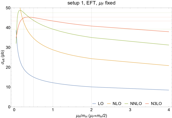
As an example, I have included the calculation of $gg\to H$ at next-to-next-to-next-to-leading order (N³LO) [2]. In Figure 2, the renormalisation scale was varied around $\mu=m_{H}/2$ . At LO ( $n=0$ ), the value was found as $19_{-4}^{+7}\,{\rm pb}$ . The next-to-leading order (NLO) ( $n=1$ ) value $43_{-8}^{+14}\,{\rm pb}$ is outside this error band but after this, the next-to-next-to-leading order (NNLO) value stabilises at $48._{-4.}^{+8.}\,{\rm pb}$ . The final value at N³LO is quoted as $44.96_{-0.10}^{+1.6}\,{\rm pb}$ .

This example demonstrates both the power and the limitation of the scale variation strategy: the LO result is completely incorrect and the error is underestimated by a factor of three. However, once the NLO corrections are taken into account (which are huge at around $K=2.2\gg\alpha_{s}=0.1$ ) the estimate becomes more reliable.

Line chart titled `setup 1, EFT, μF fixed' showing σeff pb versus μR / mH for four perturbative orders: LO, NLO, NNLO, and N3LO. All curves rise sharply at very small μR/mH, peak around 0.1 to 0.3, then decrease as μR increases. LO is lowest across the range, ending near 9 pb at 4; NLO ends near 21 pb; NNLO ends near 31 pb; and N3LO ends near 38 pb. — Figure 2: A plot of the result for the cross section for $gg\to H$ at LO, NLO, NNLO, and N³LO as a function of the renormalisation scale, here labeled $\mu_{R}$ . Figure taken from [2].

6.3 Running coupling

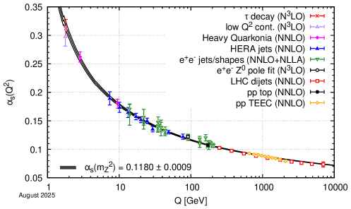
Once we have chosen the scale $\mu$ , we need to obtain a numerical value for $\alpha_{s}(\mu)$ . In principle this is easy, we can compare an observable calculated at that scale $\mathbb{O}\big{(}\alpha_{s}(\mu),\mu\big{)}$ to experimental data obtained at that scale and extract a suitable value for $\alpha_{s}(\mu)$ . However, what do we do if there is no data yet for our choice of $\mu$ ? We could of course pick a different value of $\mu$ but as we have seen from Figure 2, it is advisable to be close to the sensible scale of the process. We can therefore ask ourselves if we can relate $\alpha_{s}(\mu)$ to the value we should use at some other scale $\mu^{\prime}$ . This further allows us to combine data obtained at different $\mu$ into a global fit of $\alpha_{s}$ as perform a very stringent test of the underlying QFT. For QCD this is shown in Figure 3 with a plot taken from [15].

Running of the strong coupling αs(Q^2) as a function of the momentum scale Q in GeV, shown on a logarithmic Q-axis from about 1 to 10,000 GeV. The curve decreases smoothly from about 0.35 at low Q to about 0.075 at the highest scales. Data points from multiple measurements are overlaid, including τdecay, low-Q^2 continuum, heavy quarkonia, HERA jets, e^+e^- jets and σpole fits, LHC dijets, top-pair production, and pp TEEC, all consistent with the QCD running prediction. The reference value αs at mZ is 0.1180 +- ±0.0009 as indicated near the bottom of the plot — Figure 3: Summary of determinations of $\alpha_{s}$ as a function of the energy scale $Q$ compared to the running of the coupling computed at five loops. Taken from [15].

The theoretical description underlying this is the $\beta$ function

\displaystyle\mu^{2}\frac{\partial\alpha_{s}(\mu^{2})}{\partial\mu^{2}}=\beta% \big{(}\alpha_{s}(\mu^{2})\big{)}=-\frac{\beta_{0}}{4\pi}\alpha_{s}^{2}-\frac{% \beta_{1}}{16\pi^{2}}\alpha_{s}^{3}+\cdots\,.

(201)

To actually calculate these, we begin by noting that

\displaystyle\alpha_{s,0}(\epsilon)=\mu^{2\epsilon}Z_{g}^{2}(\epsilon,\mu^{2})% \alpha_{s}(\mu^{2})\,,

(202)

where the $\epsilon$ argument indicates that the quantity is divergent. The bare coupling $\alpha_{s,0}$ is divergent but does not depend on $\mu^{2}$ . We can therefore, its derivative w.r.t. $\mu^{2}$ therefore vanishes

\displaystyle 0=\mu^{2}\frac{\partial\alpha_{s,0}(\mu^{2})}{\partial\mu^{2}}=% \mu^{2\epsilon}Z_{g}^{2}(\epsilon,\mu^{2})\Bigg{[}\Bigg{(}\epsilon+\frac{\mu^{% 2}}{Z_{g}^{2}}\frac{\partial Z_{g}^{2}}{\partial\mu^{2}}\Bigg{)}\alpha_{s}(\mu% ^{2})+\underbrace{\mu^{2}\frac{\partial\alpha_{s}(\mu^{2})}{\partial\mu^{2}}}_% {-\beta}\Bigg{]}\,.

(203)

Solving the $[\cdots]$ for $\beta$ , we find

\displaystyle\beta\big{(}\alpha_{s}(\mu^{2})\big{)}=-\lim_{\epsilon\to 0}\frac% {\mu^{2}}{Z_{g}^{2}}\frac{\partial Z_{g}^{2}}{\partial\mu^{2}}\alpha_{s}(\mu^{% 2})\,.

(204)

If we use dimensional regularisation,

\displaystyle Z_{g}=1+\alpha_{s}(\mu^{2})\,\frac{Z_{g}^{(1)}}{4\pi\epsilon}+% \mathcal{O}(\alpha_{s}^{2},\alpha_{s}\epsilon^{0})\,.

(205)

Therefore, the first term of the $\beta$ function is just the coefficient of the pole since

\displaystyle\beta\big{(}\alpha_{s}(\mu^{2})\big{)}=-\lim_{\epsilon\to 0}\frac% {2Z_{g}^{(1)}}{4\pi\epsilon}\mu^{\frac{\partial\alpha_{s}}{\partial\mu^{2}}}% \alpha_{s}(\mu^{2})=\frac{2Z_{g}^{(1)}}{4\pi}\,.

(206)

And therefore $\beta_{0}=-2Z_{g}^{(1)}$ . The actual calculation of $Z_{g}^{(1)}$ can be performed using any quantity that involves an interaction vertex. Performing this calculation goes beyond the scope of these notes but we find in Feynman gauge (for arbitrary gauge, see for example [6])


	$\displaystyle Z_{1}^{(1)}$	$\displaystyle=-\frac{C_{F}+C_{A}}{4\pi}\,,$	(207a)
	$\displaystyle Z_{2}^{(1)}$	$\displaystyle=-\frac{C_{F}}{4\pi}\,,$	(207b)
	$\displaystyle Z_{3}^{(1)}$	$\displaystyle=-\frac{-5C_{A}+2n_{f}}{3\cdot 4\pi}\,.$	(207c)
Here $n_{f}$ is the number of active quark flavours. You can see that $Z_{1}/Z_{2}=1-\alpha/(4\pi)\ C_{A}$ which would be equal to $1$ in QED as required. Further, we can calculate $Z_{g}^{(1)}$ from $Z_{g}=Z_{1}/Z_{2}/\sqrt{Z_{3}}$

	$\displaystyle Z_{g}^{(1)}=2Z_{1}^{(1)}-2Z_{2}^{(1)}-Z_{3}^{(1)}=\frac{-11C_{A}% +2n_{f}}{24\pi}\,.$		(207d)

or equivalently

	$\displaystyle\beta_{0}$	$\displaystyle=\frac{11}{3}C_{A}-\frac{2}{3}n_{f}\,,$	(208a)
The QCD $\beta$ function is actually known up to five-loops. The next terms are
	$\displaystyle\beta_{1}$	$\displaystyle=\frac{34}{3}C_{A}^{2}-\frac{10}{3}C_{A}n_{f}-2C_{F}n_{f}\,,$	(208b)
	$\displaystyle\beta_{2}$	$\displaystyle=\frac{2857}{54}C_{A}^{3}-\frac{1415}{54}n_{f}C_{A}^{2}-\frac{205% }{18}n_{f}C_{F}C_{A}+n_{f}C_{F}^{2}+\frac{79}{54}n_{f}^{2}C_{A}+\frac{11}{9}n_% {f}^{2}C_{F}$	(208c)
	$\displaystyle\beta_{3}$	$\displaystyle=\frac{149753}{6}+3564\zeta_{3}+\Big{(}-\frac{1078361}{162}-\frac% {6508}{27}\zeta_{3}\Big{)}n_{f}+\Big{(}\frac{50065}{162}+\frac{6472}{81}\zeta_% {3}\Big{)}n_{f}^{2}+\frac{1093}{729}n_{f}^{3}$	(208d)
	$\displaystyle\beta_{4}$	$\displaystyle=\frac{8157455}{16}+\frac{621885}{2}\zeta_{3}-\frac{88209}{2}% \zeta_{4}-288090\zeta_{5}$
		$\displaystyle\qquad+\Big{(}-\frac{336460813}{1944}-\frac{4811164}{81}\zeta_{3}% +\frac{33935}{6}\zeta_{4}+\frac{1358995}{27}\zeta_{5}\Big{)}n_{f}$
		$\displaystyle\qquad+\Big{(}\frac{25960913}{1944}+\frac{698531}{81}\zeta_{3}-% \frac{10526}{9}\zeta_{4}-\frac{381760}{81}\zeta_{5}\Big{)}n_{f}^{2}$
		$\displaystyle\qquad+\Big{(}-\frac{630559}{5832}-\frac{48722}{243}\zeta_{3}+% \frac{1618}{27}\zeta_{4}+\frac{460}{9}\zeta_{5}\Big{)}n_{f}^{3}$
		$\displaystyle\qquad+\Big{(}\frac{1205}{2916}-\frac{152}{81}\zeta_{3}\Big{)}n_{% f}^{4}$	(208e)

The four- [16, 5] and five-loop [3, 9, 8, 10, 4] results are so long that I have given them here with $C_{A}=3$ and $C_{F}=4/3$ . $\beta_{0}$ and $\beta_{1}$ are independent of the renormalisation scheme chosen and the remainder is given in the $\overline{\rm MS}$ scheme.

Let us look at the first term in a bit more detail. If we solve the differential equation (201), we find

\displaystyle\alpha_{s}(\mu)=\frac{\alpha_{s}(\mu_{0})}{1-\frac{\alpha_{s}(\mu% _{0})}{4\pi}\beta_{0}\log\frac{\mu_{0}^{2}}{\mu^{2}}}\,.

(209)

A lot now depends on the sign of $\beta_{0}$ . In QED ( $C_{A}=0$ ), $\beta_{0}<0$ so $\alpha$ with $\mu$ . Even though this growth is very, very slow (at $\mu=m_{Z}$ $\alpha\approx 1/127$ once the full running is taken into account), it will eventually diverge at²² 2 Note that in QED, $n_{f}$ needs to be doubled compared to QCD because of the way colour algebra works

\displaystyle\mu=m_{e}\times{\rm e}^{\frac{3\pi}{2\alpha}}=10^{280}\,{\rm GeV}\,.

(210)

This is called the Landau pole of QED and it is ultimate proof that QED is not a complete theory of nature – which we already knew because the $Z$ boson enters at a comparatively low $90\,{\rm GeV}$ .

In QCD, $\beta_{0}>0$ for $n_{f}\leq 6$ , meaning that $\alpha_{s}$ diverges not at large $\mu$ but at small $\mu$ . This effect is called confinement and it is the reason that free quarks and gluons cannot exist. The scale of this is usually called

\displaystyle\Lambda_{\rm QCD}\approx 250\,{\rm MeV}\,.

(211)

It is no coincidence that this is similar to the mass of the lightest meson. For $\mu\gg\Lambda_{\text{\acs{QCD}}}$ QCD\mu\gg\Lambda_{\text{\acs{QCD}}}, $\alpha_{s}\ll 1$ and we can use perturbation theory. QCD is therefore said to be asymptotically free.